
1
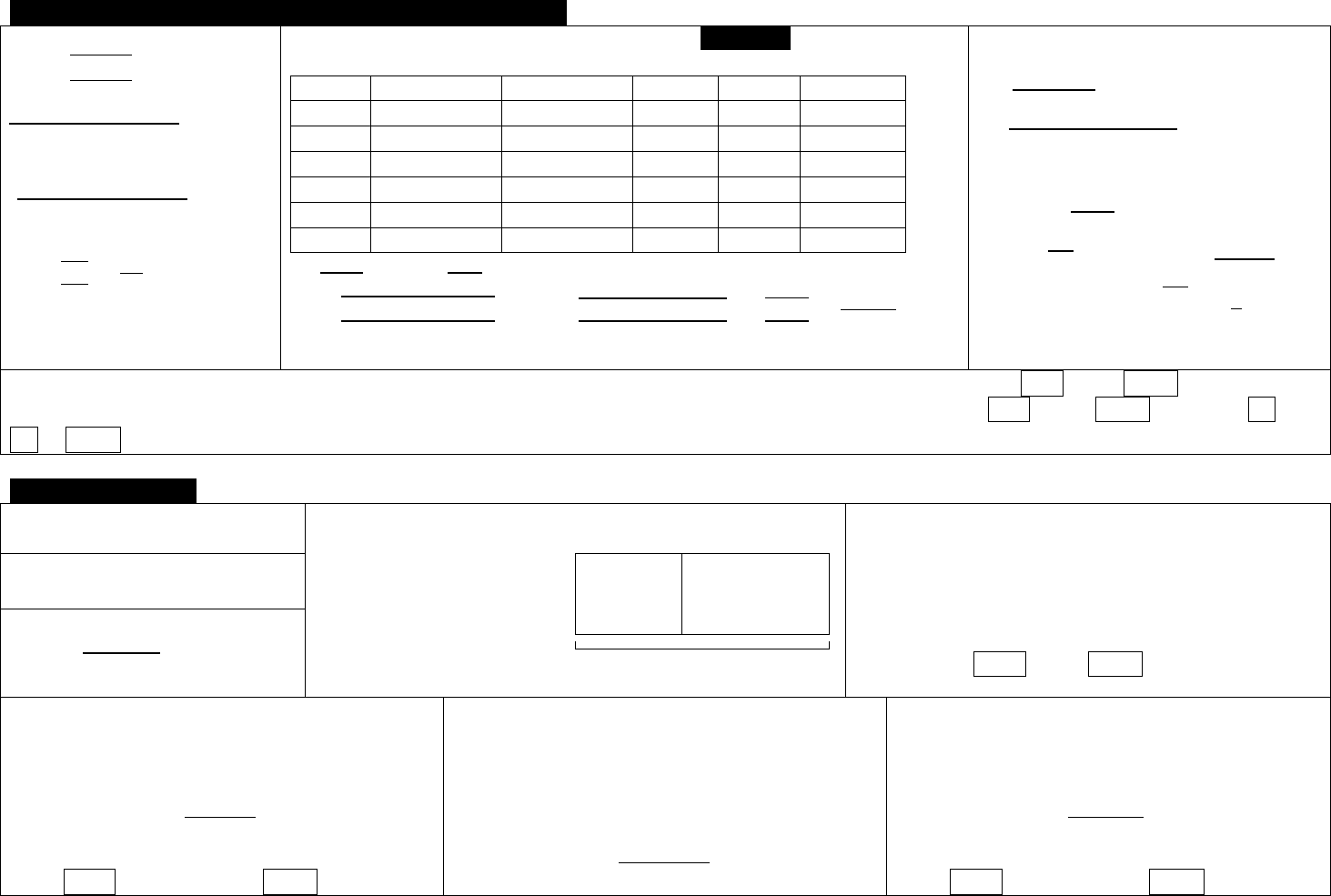
TI 83/84 Calculator – The Basics of Statistical Functions
What you
want to
do >>>
Put Data in Lists
Get Descriptive
Statistics
Create a histogram,
boxplot, scatterplot,
etc.
Find normal or
binomial probabilities
Confidence Intervals or
Hypothesis Tests
How to
start
STAT > EDIT > 1: EDIT
ENTER
[after putting data in a
list]
STAT > CALC >
1: 1-Var Stats ENTER
[after putting data in a
list]
2
nd
STAT PLOT 1:Plot 1
ENTER
2
nd
VARS
STAT > TESTS
What to do
next
Clear numbers already
in a list: Arrow up to L1,
then hit CLEAR, ENTER.
Then just type the
numbers into the
appropriate list (L1, L2,
etc.)
The screen shows:
1-Var Stats
You type:
2nd L1 or
2nd L2, etc. ENTER
The calculator will tell
you , s, 5-number
summary (min, Q1,
med, Q3, max), etc.
1. Select “On,” ENTER
2. Select the type of
chart you want,
ENTER
3. Make sure the
correct lists are
selected
4. ZOOM 9
The calculator will
display your chart
For normal probability,
scroll to either
2: normalcdf(,
then enter low value,
high value, mean,
standard deviation; or
3:invNorm(, then enter
area to left, mean,
standard deviation.
For binomial
probability, scroll to
either 0:binompdf(, or
A:binomcdf( , then
enter n,p,x.
Hypothesis Test:
Scroll to one of the
following:
1:Z-Test
2:T-Test
3:2-SampZTest
4:2-SampTTest
5:1-PropZTest
6:2-PropZTest
C:X
2
-Test
D:2-SampFTest
E:LinRegTTest
F:ANOVA(
Confidence Interval:
Scroll to one of the
following:
7:ZInterval
8:TInterval
9:2-SampZInt
0:2-SampTInt
A:1-PropZInt
B:2-PropZIn
Other points: (1) To clear the screen, hit 2
nd
, MODE, CLEAR
(2) To enter a negative number, use the negative sign at the bottom right, not the negative sign above the plus sign.
(3) To convert a decimal to a fraction: (a) type the decimal; (b) MATH > Frac ENTER
2
Frank’s Ten Commandments of Statistics
1. The probability of choosing one thing with a particular characteristic equals
the percentage of things with that characteristic.
2. Samples have STATISTICS. Populations have PARAMETERS.
3. “Unusual” means more than 2 standard deviations away from the mean; “usual” means within 2
standard deviations of the mean.
4. “Or” means Addition Rule; “and” means Multiplication Rule
5. If Frank says Binomial, I say npx.
6. If σ (sigma/the standard deviation of the population) is known, use Z; if σ is unknown, use T.
7. In a Hypothesis Test, the claim is ALWAYS about the population.
8. In the Traditional Method, you are comparing POINTS (the Test Statistic and the Critical Value); in the
P-Value Method, you are comparing AREAS (the P-Value and α (alpha)).
9. If the P-Value is less than α (alpha), reject H
0
(“If P is low, H
0
must go”).
10. The Critical Value (point) sets the boundary for α (area). The Test Statistic (point) sets the boundary
for the P-Value (area).
3
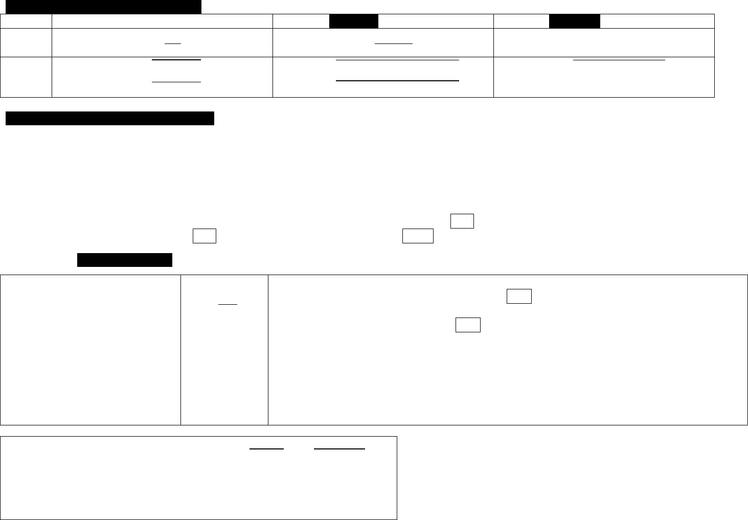
Chapters 3-4-5 – Summary Notes
Chapter 3 – Statistics for Describing, Exploring and Comparing Data
Calculating Standard Deviation
s =
Example:
x x – (x - )
2
1 -5 25
3 -3 9
14 8 64
Total 98
= 6 (18/3)
s =
=
= 7
Finding the Mean and Standard Deviation from a Frequency Distribution
Speed
Midpoint (x)
Frequency (f)
x
2
f · x
f · x
2
42-45
43.5
25
1892.25
1087.5
47306.25
46-49
47.5
14
2256.25
665
31587.50
50-53
51.5
7
2652.25
360.5
18565.75
54-57
55.5
3
3080.25
166.5
9240.75
58-61
59.5
1
3540.25
59.5
3540.25
50
2339
110240.50
=
, so
≈ 46.8
s =
, so s =
=
≈
≈ 4.1
Percentiles and Values
The percentile of value x =
(round to nearest whole number)
To find the value of percentile k:
L =
; this gives the location of
the value we want; if it’s not a whole number,
we go up to the next number. If it is a whole
number, then the answer is the mean of that
number and the number above it.
***Using the Calculator: To find mean & standard deviation of a frequency distribution or a probability distribution: First: STAT > EDIT ENTER, then in L1 put in
all the x values (midpoints if it’s a frequency distribution); in L2 put in frequencies or probabilities as applicable. Second: STAT > CALC ENTER 1-Var Stats 2
ND
L1,
2
ND
L2 ENTER. The screen shows the mean () and the standard deviation, either Sx (if it’s a frequency distribution) or σx (if it’s a probability distribution).
Chapter 4 - Probability
Addition Rule (“OR”)
P(A or B) = P(A) + P(B) – P(A and B)
Find the probability of “at least 1” girl out of 3 kids, with boys
and girls equally likely.
0 girls) =
P(all boys)
= .125*
P(at least 1 girl) =
P(1, 2 or 3 girls)
= 1 minus .125 =
.875
These are complements, so their
combined probability must = 1.
Fundamental Counting Rule: For a sequence of two
events in which the first event can occur m ways and the
second event can occur n ways, the events together can
occur a total of m · n ways.
Factorial Rule: A collection of n different items can be
arranged in order n! different ways. (Calculator Example:
To get 4!, hit 4MATH>PRB>4ENTER
Multiplication Rule (“AND”)
P(A and B) = P(A) · P(B|A)
Conditional Probability
P(B|A) =
Permutations Rule (Items all Different)
1. n different items available.
2. Select r items without replacement
3. Rearrangements of the same items are
considered to be different sequences (ABC is
counted separately from CBA)
Calculator example: n = 10, r = 8, so
10
P
8
Hit 10 MATH > PRB > 2, then 8 ENTER = 1814400
Permutations Rule (Some Items Identical)
1. n different items available, and some are
identical
2. Select all n items without replacement
3. Rearrangements of distinct items are
considered to be different sequences.
# of permutations =
Combinations Rule
1. n different items available.
2. Select r items without replacement
3. Rearrangements of the same items are
considered to be the same sequence (ABC is
counted the same as CBA)
Calculator example: n = 10, r = 8, so
10
C
8
Hit 10 MATH > PRB > 3, then 8 ENTER = 45
*“All boys” means #1 is a boy
AND #2 is a boy AND #3 is a
boy, so we use the
Multiplication Rule:
.5 x .5 x .5 = .125
4
Formulas for Mean and Standard Deviation
All Sample Values
Frequency Distribution
Probability Distribution
Mean
Std Dev
Chapter 5 - Discrete Probability Distributions
Sec. 5.2
A random variable is simply a number that can change, based on chance. It can either be discrete (countable, like how many eggs a hen might lay), or
continuous (like how much a person weighs, which is not something you can count). Example: The number of Mexican-Americans in a jury of 12 members is a
random variable; it can be anywhere between 0 and 12. And it is a discrete random variable, because it is a number you can count.
To find the mean and standard deviation of a probability distribution by hand, you need 5 columns of numbers: (1) x; (2) P(x); (3) x · P(x); (4) x
2
; (5) x
2
· P(x).
Using the Calculator: To find the mean and standard deviation of a probability distribution, First: STAT > EDIT, then in L1 put in all the x values, and in L2 put in
the probability for each x value. Second: STAT > CALC > 1-Var Stats > 1-Var Stats L1, L2 ENTER.
Sec. 5.3 – 5.4 – Binomial Probability
Requirements
___ Fixed number of trials
___ Independent trials
___ Two possible outcomes
___ Constant probabilities
Formulas
µ = n · p
q = 1 - p
Using the Calculator
1. To get the probability of a specific number: 2
nd
VARS binompdf (n, p, x) (which gives you the
probability of getting exactly x successes in n trials, when p is the probability of success in 1 trial).
2. To get a cumulative probability: 2
nd
VARS binomcdf (n, p, x) (which gives you the probability of
getting up to x successes in n trials, when p is the probability of success in 1 trial). IMPORTANT:
there are variations on this one, which we will talk about. Be sure to get them clear in your mind.
At most/less than or equal to: ≤ binomcdf(n,p,x)
Less than: < binomcdf(n,p,x-1)
At least/greater than or equal to: ≥ 1 minus binomcdf(n,p,x-1)
Greater than/more than: > 1 minus binomcdf(n,p,x)
Symbol Summary Sample Population
How many?
n N
Mean
µ
Proportion
p
Standard Deviation
s
Correlation Coefficient
r
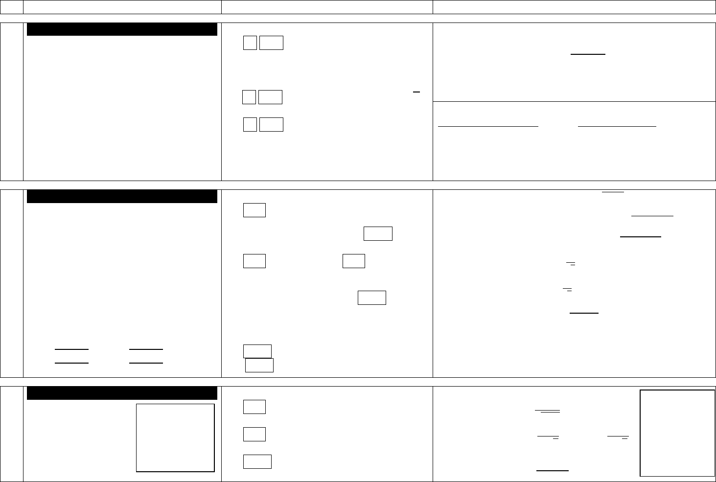
5
Chapters 6-7-8 – Summary Notes
Ch
Topic
Calculator
Formulas, Tables, Etc.
6
Normal Probability Distributions
3 Kinds of problems:
1. You are given a point (value) and
asked to find the corresponding area
(probability)
1a. Central Limit Theorem. Just like #1,
except n > 1.
2. You are given an area (probability) and
asked to find the corresponding point
(value).
3. Normal as approximation to binomial
1. 2
nd
VARS normalcdf (low, high, µ,σ)
1a. 2
nd
VARS normalcdf (low, high, µ ,
)
2. 2
nd
VARS invNorm (area to left, µ, σ)
3. Step 1: Using binomial formulas, find
mean and standard deviation.
Table A-2.
3. (cont’d – Normal as approximation to binomial) – Step 2:
If you are asked to find Then in calculator
P(at least x) normalcdf(x-.5,1E99,µ,σ)
P(more than x) normalcdf(x+.5,1E99,µ,σ)
P(x or fewer) normalcdf(-1E99,x+.5,µ,σ)
P(less than x) normalcdf(-1E99,x-.5,µ,σ)
7
Confidence Intervals
1. Proportion
2. Mean (z or t?)
3. Standard Deviation
< σ <
1. STAT > TEST > 1PropZInt
Minimum Sample Size: PRGM NPROP
2. STAT > TEST > ZInt OR STAT > TEST > TInt
(use Z if σ is known, T if σ is unknown)
Minimum Sample Size: PRGM NMEAN
3. PRGM >INVCHISQ (to find
and
)
PRGM > CISDEV (to find Conf. Interval.)
1. = sample proportion; E = z
α/2
Min. Sample Size ( unknown):
Min. Sample Size ( known):
2. = sample mean; E = z
α/2
(σ known)
or E = t
α/2
(σ unknown)
Min. Sample Size: n =
3. Use Table A-4 to find
and
8
Hypothesis Tests
1. Proportion
2. Mean (z or t?)
3. Standard Deviation
1. STAT > TEST > 1PropZTest
2. STAT > TEST > ZTest OR TTest
3. PRGM > TESTSDEV
1. Test Statistic: z =
2. Test Statistic: z =
OR t =
3. Test Statistic: X
2
=
If P-Value < α,
reject H
0;
if P-
Value > α fail
to reject H
0
.
See additional
sheet on 1-
sentence
statement and
finding Critical
Value.
6
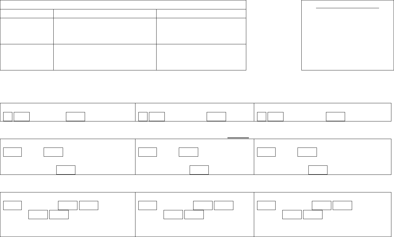
Hypothesis Tests
1-Sentence Statement/Final Conclusion
Hypoth Test Checklist
___ CLAIM
___ HYPOTHESES
___ SAMPLE DATA
___ α
___ CALCULATOR: P-VALUE,
TEST STATISTIC
___ CONCLUSIONS
Claim is H
0
Claim is H
1
Reject H
0
(Type
1 – reject true
H
o
)
There is sufficient evidence to
warrant rejection of the claim
that . . .
The sample data support the
claim that . . .
Fail to reject H
0
(Type II – fail to
reject false H
o
)
There is not sufficient evidence
to warrant rejection of the claim
that . . .
There is not sufficient
sample evidence to support
the claim that . . .
To find Critical Value
(required only for Traditional Method, not for P-Value Method)
Critical Z-Value
Left-Tail Test (1 negative CV)
2
nd
VARS invNorm(α) ENTER
Right-Tail Test (1 positive CV)
2
nd
VARS invNorm(1-α) ENTER
Two-Tail Test (1 neg & 1 pos CV)
2
nd
VARS invNorm(α/2) ENTER
Critical T-Value (when you get to Chapter 9, for TWO samples, for DF use the smaller sample)
Left-Tail Test (1 negative CV)
PRGM > INVT ENTER
AREA FROM LEFT = α
DF = n-1 ; then hit ENTER
Right-Tail Test (1 positive CV)
PRGM > INVT ENTER
AREA FROM LEFT = 1-α
DF = n-1; then hit ENTER
Two-Tail Test (1 neg & 1 pos CV)
PRGM > INVT ENTER
AREA FROM LEFT = α/2
DF = n-1; then hit ENTER
Critical X
2
-Value
Left-Tail Test (1 positive CV)
PRGM > INVCHISQ ENTER ENTER
DF = n-1 ENTER ENTER
AREA TO RIGHT = 1 - α
Right-Tail Test (1 positive CV)
PRGM > INVCHISQ ENTER ENTER
DF = n-1 ENTER ENTER
AREA TO RIGHT = α
Two-Tail Test (MUST DO TWICE)
PRGM > INVCHISQ ENTER ENTER
DF = n-1 ENTER ENTER
AREA TO RIGHT: 1
st
time: α/2 (
)
2
nd
time: 1 - α/2 (
)
7
Chapters 9-10-11 – Summary Notes
Chapter 9 – Inferences from Two Samples (Be sure to use Hypothesis Test Checklist)
Proportions (9-2)
Means (9-3) (independent samples)
Matched Pairs (9-4) (dependent samples)
Hypothesis Test
(Be sure to use Hypoth
Test checklist)
Calculator: 2-PropZTest
Formulas:
H
0
: p
1
= p
2
; H
1
: p
1
< or > or ≠ p
2
Calculator: 2-SampleTTest
H
0
: µ
1
= µ
2
; H
1
: µ
1
< or > or ≠ µ
2
Calculator: (1) Enter data in L1 and L2, L3
equals L1 – L2; (2) TTest (which gives you all the
values you need to plug into the formula)
H
0
: µ
d
= 0; H
1
: µ
d
< or > or ≠ 0
Confidence Interval
Calculator: 2-PropZInt.
Calculator: 2-SampleTInt
Calculator: TInterval
No formulas. If interval contains 0, then fail to reject. If for a 1-tail Hypo. Test is .05, the CL for Conf. Int. is 0.9 (1 - 2).
Chapter 10 – Correlation and Regression (don’t use formulas, just calculator; the important thing is interpreting results.)
Question to be answered
Calculator and Interpretation (Anderson: show value of t but not formula)
Hypothesis Test: Is there a linear
correlation between two variables,
x and y? (10-2)
r is the sample correlation
coefficient. It can be between -1
and 1.
Calculator: Enter data in L1 and L2, then STAT > Test > LinRegTTest. (Reg EQ > VARS, Y-VARS, Function, Y1). P-Value tells
you if there is a linear correlation. The test statistic is r, which measures the strength of the linear correlation.
Interpretation: x is the explanatory variable; y is the response variable. H
0
: there no linear correlation; H
1
: there is a linear
correlation. So, if P-Value < , you reject H
0,
so there IS a linear correlation; if P-Value > , you fail to reject H
0,
so there is
NO linear correlation.
Calculator: To create a scatterplot: Enter data in L1 and L2, then LinRegTTest; then 2
nd
Y = Plot 1 On, select correct type
of plot. Then Zoom 9 (ZoomStat). To delete regression line from graph, Y= , then clear equation from Y1.
When you have 2 variables x and y,
how do you predict y when you are
given a particular x-value? (10-3)
Two possible answers:
(1) If there is a significant linear correlation, then you need to determine the Regression Equation (y = a + bx; LinRegTTest
gives you a and b), then just plug in the given x-value. Or the easy way to find y for any particular value of x:
Calculator: VARS Y-Vars 1:Function Enter Enter Input x-value in parentheses after Y1
(2) If there is no significant linear correlation, then the best predicted value for y = . Calculator: VARS, 5, 5, ENTER.
When you have 2 variables x and y,
how do you predict an interval
estimate for y when you are given
a particular x-value? (10-4)
1. PROGRAM, INVT ENTER Area from left is 1-/2, DF = n-2. This gives you t Critical Value.
2. PROGRAM, PREDINT ENTER Input t Critical Value from Step 1, then input X value given in the problem. Hit Enter twice
to get the Interval.
How much of the variation in y is
explained by the variation in x?
(10-4)
The percentage of variation in y that is explained by variation in x is r
2
, the coefficient of determination.
Calculator: to find r
2
, enter data in L1 and L2, then LinRegTTest. It will give you r
2
. 1 sentence conclusion: “[r
2
]% of the
variation in [y-variable in words] can be explained by the variation in [x-variable in words].”
Total Variation is
. Explained Variation is Total Variation times r
2
. Unexplained Variation is Total Variation
minus Explained Variation. To find them all, put x values in L1; put y values in L2; LinRegTTest; then PRGM VARATION.
µ
1
- µ
2
always = 0
µ
d
always = 0
p
1
– p
2
always = 0.

8
Chapter 10 - continued
Finding Total Deviation,
Explained Deviation, and
Unexplained Deviation,
for a point. (10-4)
Variation and Deviation are similar, but different. Variation relates to ALL the points in a set of correlated data. Deviation
relates to ONE specific point in a set of correlated data. Total Deviation for a specific point = (the actual y-
coordinate of the point minus the mean of all the y values). Explained Deviation for the point = (the predicted value
of y when the x-coordinate of that point is plugged into the regression equation, minus the mean of all the y values).
Unexplained Deviation for the point = (the actual y-coordinate of the point minus the predicted value of y when the
x-coordinate of that point is plugged into the regression equation).
Chapter 11 – Chi-Square (X
2
) Problems (Hypothesis Tests, use checklist)
Claim to be tested
Calculator
Formulas, etc.
The claim that an observed
proportion (O) < or = or > an
expected proportion (E). This
is called “goodness of fit.”
(11-2) *3 SAMPLES WITH
PROPORTION*
Enter O data in L1 and E data in L2.
PROGRAM BESTFIT ENTER
Enter number of categories (k),
then Enter,
Gives you Chi-Square (X
2
) and P-
Value
Two types of claims: equal proportions or unequal proportions:
Equal: H
0
: p
1
=p
2
=p
3
; H
1
: at least one is not equal
Unequal: H
0
: p
1
=.45, p
2
= .35, p
3
= .20; H
1
: at least one is not equal to the claimed
proportion
Test Statistic is X
2
(Chi-Square)
2
=
Given a table of data with
rows and columns, the claim
that the row variable is
INDEPENDENT of the column
variable. This is called
“contingency tables.” (11-3)
2
nd
MATRX EDIT, select [A], make
sure number of rows and number
of columns are correct, then enter
the values in the matrix.
STAT Tests, X
2
– Test; Observed is
[A] and Expected is [B], hit Calc; it
gives you X
2
and P-Value.
Example hypotheses: H
0
: pedestrian fatalities are independent of intoxication of driver ;
H
1
: pedestrian fatalities depend
on intoxication of driver.
2
=
To find X
2
CV, df = (r-1)(c-1).
Chapter 11 – Analysis of Variance (ANOVA) (Hypothesis Tests, use checklist)
Claim to be tested
Calculator
Formulas, etc. (must show formulas in both symbolic form and also with
given data plugged in, but can get the answer from calculator)
The claim that 3 or more
population means are all
equal (H
0
), or are not all equal
(H
1
). This is called “Analysis
of Variance.” (11-4) * 3
SAMPLES WITH MEAN*
Enter data in L1, L2, etc.
STAT Tests, ANOVA (L1, L2, L3). Gives you F
and PV, but also gives you Factor: df, SS and
MS, and Error: df, SS and MS, which you need
to plug into the formula.
The test statistic is F. H
0
:
1
=
2
=
3
; H
1
: at least one mean is not equal.
F = SS Factor
df = MS Factor
SS Error MS Error
df
MS(total)=SS(total)/(N-1). N=total number of values in all samples combined
E (the expected value) for any cell = (row total x
column total) / grand total, OR get all E-values on
calculator with 2
nd
MATRX Edit [B] Enter
SS stands for “Sum of Squares”
MS stands for “Mean Squares”
Hypothesis Test is always right-tail
To find P-Value from Test Stat: X
2
cdf(TS,1E99,k-1)

9
Overview of Chapters 7, 8 and 9
ONE-Sample Problems
TWO-Sample Problems
Chapter 7
Chapter 8
Chapter 9
Type of
Problem
Confidence Interval
Hypothesis Test
Type of Problem
Confidence
Interval
Hypothesis Test
Proportion
1-Prop Z Int
1-Prop Z Test
Proportion
2-Prop Z Int
2-Prop Z Test
Mean –
σ known
Z Interval
Z Test
Mean –
Independent
Samples
2-Samp T Int
2-Samp T Test
Mean –
σ unknown
T Interval
T Test
Standard
Deviation
PRGM S2INT (Toma);
or
PRGM INVCHISQ +
PRGM CISDEV
PRGM S2TEST (Toma);
or
PRGM TESTSDEV
Mean –
Dependent
Samples
(Matched Pairs)
T Interval
T Test
Minimum Sample Size Problems (Chapter 7)
Chapter 7 also has another kind of problem, called Minimum Sample Size Problems.
These problems may ask you to find the minimum sample size, but usually they just say “How many . . .?”
Minimum Sample Size problems can be Proportion problems, Mean problems or Standard Deviation problems.
Proportion problems: Use PRGM NPROP. This program asks you for SAMPLE P. If the problem gives you a Sample P (like 60%), then just
enter that, as a decimal. If the problem does NOT give you a Sample P, then enter 0.5.
Mean problems: Use PRGM NMEAN.
Both programs (NPROP and NMEAN) ask you for the Margin of Error. Sometimes the Margin of Error is clear from the problem. But if you see the
word “within” in the problem, the margin of error is whatever comes immediately after the word “within.”
Standard Deviation problems: You are very rarely asked to find the Minimum Sample Size for a Standard Deviation problem. The only way
to answer this kind of problem is by looking at the table in the Triola Text, which is on page 364 of the 4th Edition.

10
Finding the key words in a problem (Ch. 6, 7 and 8)
Sample Problem
Key Words
Sample
Statistics
1. Assume that heights of men are normally distributed, with
a mean of 69.0 in. and a standard deviation of 2.8 in. A day
bed is 75 in. long. Find the percentage of men with heights
that exceed the length of a day bed.
“normally distributed” tells you it’s probably a Ch. 6 question.
“Find the percentage” tells you it’s a Type 1 Ch. 6 question (use normalcdf)
NA
2. Assume that heights of men are normally distributed, with
a mean of 69.0 in. and a standard deviation of 2.8 in. In
designing a new bed, you want the length of the bed to
equal or exceed the height of at least 95% of all men.
What is the minimum length of this bed?
“normally distributed” tells you it’s probably a Ch. 6 question.
“What is the minimum length” tells you it’s NOT a Type 1 Ch. 6 question, so it’s
a Type 2 Ch. 6 question (use invNorm)
NA
3. The cholesterol levels of men aged 18-24 are normally
distributed with a mean of 178.1 and a standard deviation
of 40.7. If 1 man aged 18-24 is randomly selected, find the
probability that his cholesterol level is greater than 260.
“normally distributed” tells you it’s probably a Ch. 6 question.
“Find the probability” tells you it’s a Type 1 Ch. 6 question (use normalcdf)
NA
4. In a poll of 745 randomly selected adults, 589 said that it
is morally wrong to not report all income on tax returns.
Construct a 95% confidence interval estimate of the
percentage of all adults who have that belief.
“poll” and “randomly selected” both tell you the sentence is about a sample.
“Construct a confidence interval” tells you you’re constructing a confidence
interval (Ch. 7), NOT testing a hypothesis (Ch. 8).
“Percentage” tells you it’s a proportion problem, not a mean or standard
deviation problem.
n = 745
x = 589
5. You must conduct a survey to determine the mean income
reported on tax returns. How many randomly selected
adults must you survey if you want to be 99% confident
that the mean of the sample is within $500 of the true
population mean?
“How many” tells you you are finding a minimum sample size.
“Mean” tells you you’re finding a minimum sample size for a mean, not for a
proportion.
“Within” tells you that the next thing you see ($500) is the margin of error.
NA
6. A simple random sample of 37 weights of pennies has a
mean of 2.4991g and a standard deviation of 0.0165g.
Construct a 99% confidence interval estimate of the mean
weight of all pennies.
“Construct a confidence interval” tells you’re constructing a confidence interval
(Ch. 7), NOT testing a hypothesis (Ch. 8).
“Mean” tells you you’re constructing a confidence interval for a mean, not for a
proportion.
The phrase “and a standard deviation” is in a sentence about the sample, so
you know the sample standard deviation (s), but you don’t know the population
standard deviation (σ), so you will use t, not z.
n = 37
s = 0.0165

11
7. The Town of Newport has a new sheriff, who compiles records
showing that among 30 recent robberies, the arrest rate is 30%,
and she claims that her arrest rate is higher than the historical
25% arrest rate. Test her claim.
“Records” tells you you are getting information about a sample.
“Rate” tells you that this is a proportion problem, not a mean problem
or standard deviation problem.
“Claim” and “Test her claim” tell you that this is a Hypothesis Test (Ch.
8) not a Confidence Interval (Ch. 7).
n = 30
= 9
8. The totals of the individual weights of garbage discarded by 62
households in one week have a mean of 27.443 lb. Assume that
the standard deviation of the weights is 12.458 lb. Use a 0.05
significance level to test the claim that the population of
households as a mean less than 30 lb.
“Assume” tells you that the standard deviation you are being given is a
population standard deviation (σ), so you will use z, not t.
“Test the claim” tell you that this is a Hypothesis Test (Ch. 8) not a
Confidence Interval (Ch. 7).
“Mean” tells you you are testing a claim about a mean, not about a
proportion or standard deviation.
“Significance level” is α (alpha)
n = 62
α = 0.05

12
Chapter 8 - Frank’s Claim Buffet
The Claim in Words
Claim Buffet
1. Test the claim that less than ¼ of such adults smoke.
P
µ
σ
>
<
≠
=
Some
number =
.25
2. Test the claim that most college students earn
bachelor’s degrees within 5 years
P
µ
σ
>
<
≠
=
Some
number =
.5
3. Test the claim that the mean weight of cars is less than
3700 lb
P
µ
σ
>
<
≠
=
Some
number =
3700
4. Test the claim that fewer than 20% of adults consumed
herbs within the past 12 months.
P
µ
σ
>
<
≠
=
Some
number =
.20
“most”
just
means
more
than half
20% tells
you the
claim is
about a
proportion

13
5. Test the claim that the thinner cans have a mean axial
load that is less than 282.8 lb
P
µ
σ
>
<
≠
=
Some
number =
282.8
6. Test the claim that the sample comes from a population
with a mean equal to 74.
P
µ
σ
>
<
≠
=
Some
number =
74
7. Test the claim that the standard deviation of the
weights of cars is less than 520.
P
µ
σ
>
<
≠
=
Some
number =
520
